Chapter 3: Sampling the Imaginary

Suppose we have a test for condition \(X\). The test correctly detect \(X\) \(95\%\) of the time. In mathematical notation, \(\Pr(\text{positive} \mid X)=0.95\). We also know that \(1\%\) of the time, the test records a false positive, i.e. \(\Pr(\text{positive} \mid \neg X)=0.01\).

To determine the probability of \(X\), given a positive test result, we can use Bayes’ theorem:

\[ \Pr(X \mid \text{positive})=\frac{\Pr(\text{positive} \mid X)\Pr(X)}{\Pr(\text{positive})} \]

\(\Pr(X)\) is the incidence of \(X\), which is known to be \(0.1\%\).

Show code

pr_p_x = 0.95
pr_p_negx = 0.01
pr_x = 0.001
pr_p = pr_p_x * pr_x + pr_p_negx * (1 - pr_x) # marginal likelihood
pr_x_p = pr_p_x * pr_x / pr_p
print(f"Probability of X: {pr_x_p:.4f}")

Probability of X: 0.0868

This means that the probability \(X\) with one positive test is only 0.868.

With two positive tests, the probability soars to > 90%, demonstrating why many medical test require two positive results:

Show code

pr_pp = pr_p_x ** 2 * pr_x + pr_p_negx ** 2 * (1 - pr_x) # marginal likelihood
pr_x_pp = pr_p_x ** 2 * pr_x / pr_pp
print(f"Probability of X: {pr_x_pp:.4f}")

Probability of X: 0.9003

But that was mathy, and we can get more intuitive by thinking in counts:

100,000 people exist in the population
So, 100 have \(X\) (\(0.1\%\)).
Of the 100 that have \(X\), 95 will test positive (\(95\%\)).
Of the 99,900 people that do not have \(X\), 999 will test positive for \(X\) (\(1\%\))

This simplifies the math wonderfully:

\[ \Pr(X \mid \text{positive}) = \frac{95}{95+999} = \frac{95}{1094} \approx 0.0868 \]

And for two positive tests, we can follow a similar counting pattern:

Of the 95 people with \(X\) who tested positive, approximately 90 will test positive again.
Of the 999 people who do not have \(X\) but tested positive, approximately 10 will test positive again.

So, the math for two positive tests is:

\[ \Pr(X \mid \text{positive}) \approx \frac{90}{90+10} = \frac{90}{100} = 0.90 \]

Why counts?

Counting is easier than calculus, even for statisticians
Bayesian analysis involves sampling, and analysis of sampling frequencies (counts). Frequencies are easy for humans to interpret - we encounter and process counts frequently.

3.1: Sampling from a grid-approximate posterior

Recall the sampler from chapter 2:

Show code

import numpy as np
import scipy.stats as st

W = 6
L = 3
p_grid = np.linspace(0, 1, num=1000)
prob_p = np.repeat(1.0, 1000)
prob_data = st.binom.pmf(W, W + L, p_grid)
posterior = prob_data * prob_p
posterior = posterior / np.sum(posterior)

After running the sampler, we are left with p, representing the posterior distribution.

We can sample from the posterior distribution to replicate a posterior density:

Show code

# Sample from the posterior
p_sample = np.random.choice(p_grid, size=10000, replace=True, p=posterior)

# Plot the results
import arviz as az
from matplotlib import pyplot as plt

x0 = np.linspace(0, len(p_sample), num=len(p_sample))
x1 = np.linspace(0, 1)
fig, (ax_samples, ax_density) = plt.subplots(1, 2, figsize=(9, 5))

ax_samples.scatter(x0, p_sample, alpha=0.25)
ax_samples.set_xlabel("Sample index")
ax_samples.set_ylabel("p")

az.plot_kde(p_sample)
ax_density.set_xlabel("p")
ax_density.set_ylabel("density")

fig.tight_layout()
plt.show()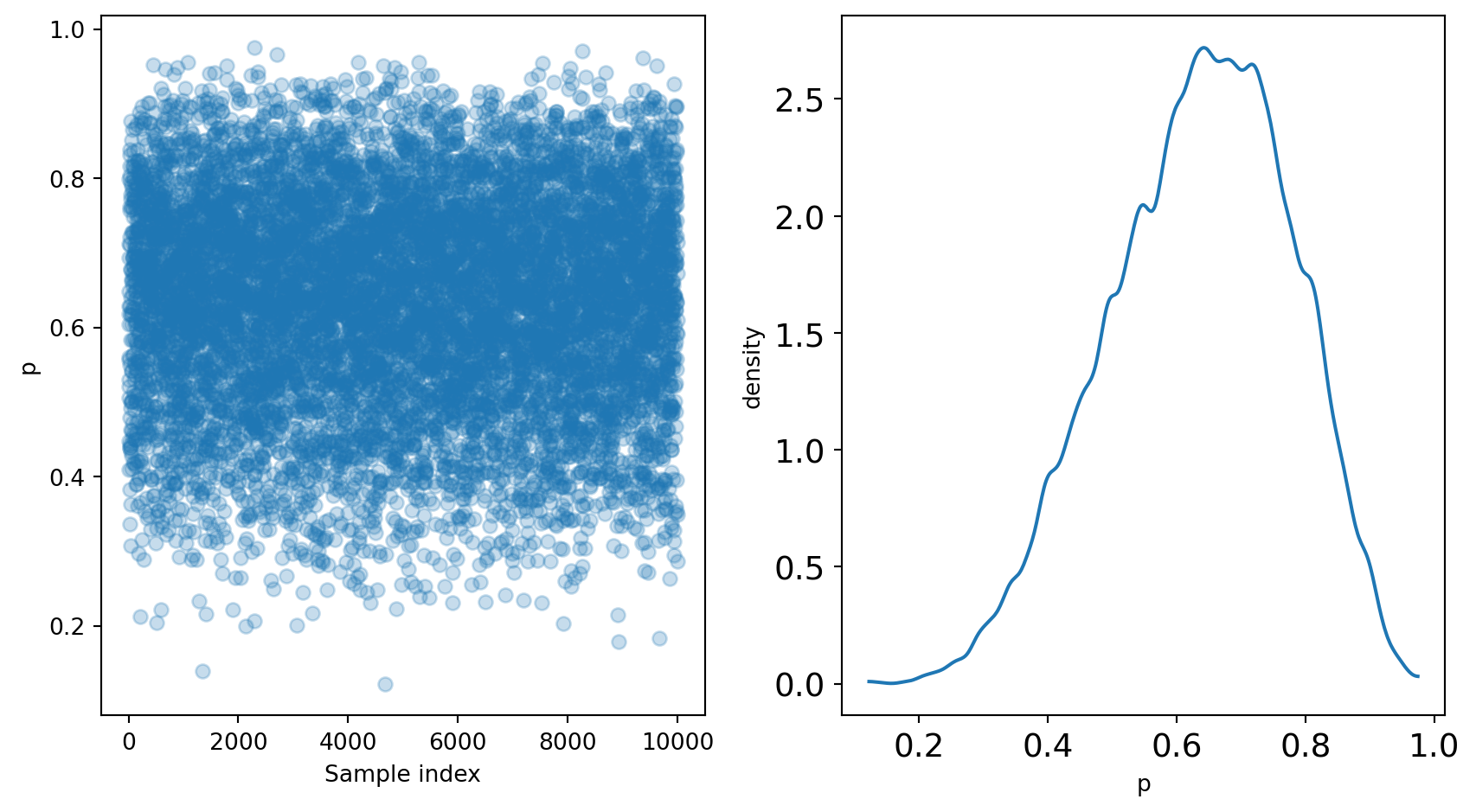

These samples can be used to further analyze the posterior.

3.2: Sampling to summarize

Summarizations of the posterior distribution can broadly be divided into three categories:

Intervals of defined boundaries
Intervals of defined probability mass
Point estimates

3.2.1: Intervals of defined boundaries

An example of such a question is “What is the chance that less than 50% of the Earth is covered in water?” This question can be answered using samples of the posterior:

Show code

prob = np.sum(posterior, where=p_grid < 0.5)
print(f"Pr(p < 0.5) = {prob:.4f}")

Pr(p < 0.5) = 0.1719

Using the grid-approximation method, we see that 17% of the posterior distribution is below 0.5.

Since grid-approximation is generally not practical, it’s useful to see that a similar result can be achieved directly from the samples of the posterior:

Show code

prob_from_samples = np.sum(p_sample < 0.5) / len(p_sample)
print(f"Pr(p < 0.5) = {prob_from_samples:.4f}")

Pr(p < 0.5) = 0.1809

The takeaway here is that sampling from the posterior is both efficient and effective.

3.2.2: Intervals of defined mass

Sometimes you want to know the “bottom 25%” or “middle 50%.” These are intervals of defined mass.

Percentile intervals are an example of intervals of defined mass:

Show code

lower_bottom25 = np.quantile(p_sample, 0)
upper_bottom25 = np.quantile(p_sample, 0.25)
print(f"Bottom 25%: ({lower_bottom25:.4f} ,{upper_bottom25:.4f})")

Bottom 25%: (0.1221 ,0.5395)

Show code

lower_middle50 = np.quantile(p_sample, 0.25)
upper_middle50 = np.quantile(p_sample, 0.75)
print(f"Middle 50%: ({lower_middle50:.4f} ,{upper_middle50:.4f})")

Middle 50%: (0.5395 ,0.7387)

You can also compute the highest posterior density interval (HPDI), which captures the interval with the highest posterior probability. While percentile intervals are evenly spaced around the point estimates, HPDI’s are not necessarily so.

Show code

hpdi_50 = az.hdi(p_sample, hdi_prob=0.50)
print(f"50% HPDI: ({hpdi_50[0]:.4f} ,{hpdi_50[1]:.4f})")

50% HPDI: (0.5746 ,0.7698)

3.2.3: Point estimates

There are several types of point estimates useful in Bayesian analysis.

The parameter with the highest posterior probability is the maximum a posteriori (MAP) estimate.

Show code

map_p = p_grid[np.argmax(posterior)]
print(f"MAP: {map_p:.4f}")

MAP: 0.6667

This can be achieved on the samples from the posterior as well.

Show code

map_p_sample = st.mode(p_sample)[0]
print(f"MAP (sampled): {map_p_sample:.4f}")

MAP (sampled): 0.6286

Of course, mean and median are also available point estimates.

Show code

print(f"mean: {np.mean(p_sample):.4f}")
print(f"median: {np.median(p_sample):.4f}")

mean: 0.6351
median: 0.6446

The choice of estimate is yours!

One way to compare the point estimates is to use a loss function, which determines the cost of any one point estimate. It is important to note that different loss functions imply different estimates, so it is best to consider multiple. Absolute loss implies the posterior median and quadratic loss implies the posterior mean.

3.3: Sampling to simulate prediction

Simulating data and scenarios using a model has several benefits:

Model design
Model checking
Software validation
Research design
Forecasting

3.3.1: Dummy data

Your can “run simulations” directly on the posterior by sampling it:

Show code

# run 100 simulations
size = 100
n = 9
p = 0.71
samples = st.binom.rvs(n=n, p=p, size=size)
fig, ax = plt.subplots(1, 1)
ax.hist(samples, bins=7, edgecolor="black")
ax.set_title(f"Results from {n} globe tosses ({size} simulations)")

Text(0.5, 1.0, 'Results from 9 globe tosses (100 simulations)')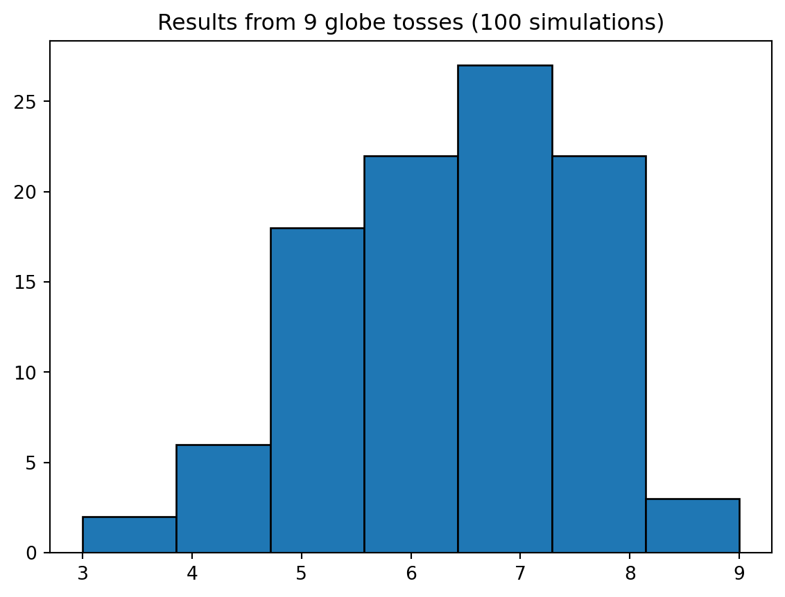

3.3.2: Model checking

Model checking involves two parts:

Ensuring the model properly fit
Ensuring the model’s usefulness

3.3.2.1: Did the software work?

One way to check model fit is through retrodictions, which involve using the original source data to generate predictions, and checking the resulting data for likeness.

3.3.2.2: Is the model adequate?

In this step, the goal is to determine how the model fails to describe the data, keeping in mind that all models are false.

Information loss is so incredibly tempting when evaluating model adequacy. The allure of a point estimate like rmse (“Look, boss! Number down!”) is almost inescapable.

Not in Bayesian analysis. Bayesian analysis utilizes the entire posterior, for not only all observations, but all samples also. If we use the entire posterior, we lose no information.

When you take the full information of the parameters, and propagate it through to the full information of the observations, you arrive at the posterior predictive distribution, illustrated in the animation from Lecture 2.